Guides
Maximizing energy arbitrage with Price-Quantity Bidding
An improved optimization method to maximize energy arbitrage in dynamic energy markets.
Energy prices are anything but regular and easy to predict. They can dip or spike suddenly and unexpectedly, fluctuate within each hour – even when trending in a consistent direction, and the timing of these shifts varies each day.
Operators that maximize arbitrage in this volatile market also maximize revenue capture. Tyba recently rolled out an enhanced bidding algorithm – Dynamic Price-Quantity (PQ) Bidding – that enables energy storage assets to maximize operating revenue by making price the determinant of how much the battery sells or discharges at any point.
How it works:
Fundamentally, there is always some price at which we are willing to charge or discharge. This approach figures out how much capacity we are willing to commit at given price levels. Specifically, for each operating interval, Tyba’s optimizer looks at the battery’s state of charge (SOC) and assesses the future buying and selling opportunities based on forecasts. It then configures and places multiple bids that offer a specific capacity for a given price.
- For example, we may be willing to discharge 30MW if prices are $50-100, 60MW from $101-$500 and 100MW for anything over $501.
Doing this enables an asset to place opportunistic bids, and capture additional value if the prices happen to be high/low enough.
Why it is advantageous
At its core, Dynamic PQ Bidding unlocks higher revenue outcomes. Especially in markets where the peaks and troughs are hard to predict. With our approach:
- Price becomes the determinant of how much energy you are willing to buy or sell, rather than quantity-based scheduling.
- Dynamically update bids based on evolving market conditions, asset state, upcoming obligations, and forecasted opportunities.
- Optimize revenue capture by selling the most capacity into the highest peaks, and charging into the lowest dips.
The majority of assets operating today take less nuanced approaches. They typically bid to fully clear or stay out of the market, and/or reuse the same PQ pairs hour-over-hour. These legacy approaches leave little flexibility to take advantage of unexpected price dips/spikes.
A few instances where Dynamic PQ Bidding helps deliver additional revenue
Examples from live energy storage operations in ERCOT.
[1] Catching an unexpected price spike
When forecasts predict that prices will likely rise in a certain time period, Dynamic PQ Bidding helps ensure the asset sells the most capacity into the highest peak. Here, we see the optimizer:
- Prepare for the spike: In each interval leading up to the spike, the optimizer evaluates the upcoming price and the most current view of all pre-spike prices. It places bid pairs that aim to charge at the lowest available prices to get to full SOC prior to the peak.
- Maximize discharge at the peak: During the peak window, we submitted ~3 discharge offers in each interval of the price spike to ensure we dispatch more energy when the prices are the highest.
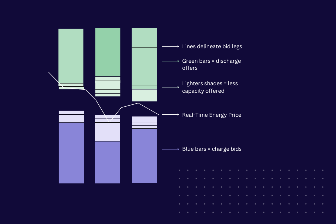
How to interpret the chart:
- Green bars represent discharge offers, and blue bars represent charge bids. Darker shades connote more capacity.
- Within the bars, the small, horizontal black lines mark where the offer pairs change. If a green bar has two black lines, it means we submitted three PQ pairs for that interval.
- The long black line that travels across the length to the chart represents forecasted prices for intervals after the current operating interval, and actual prices for trailing hours.
- If the long black (price) line intersects with a bar, that means the offer cleared.
For each interval, the bid pairs are generated in the moments before submissions are due so they account for the most up-to-date information and conditions. Each of these visuals are backward looking and highlight the bids/offers that were placed.
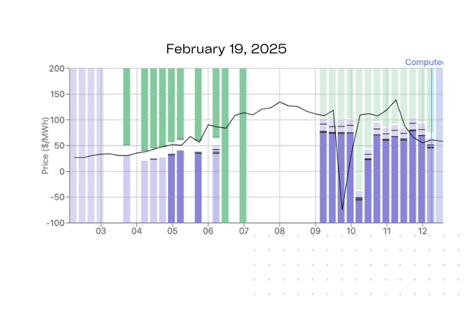
[2] Advantageous charging
If there is a forecasted spike in the future, say IE19, the asset will want to charge up to max capacity prior. If you are in IE10 now, there are 9 hours that the optimizer has to try and get a charge price below the forecasted lowest interval. It may want to place a series of PQ bids to try and pick up the lowest priced charges along the way.
Something along these lines happened on February 19th. Prices suddenly dropped at IE945 due to congestion. Staying in the market for charges caught a huge negative dip in prices, allowing us to charge up at -$87.86 and $23.
What’s more, we were able to immediately sell this energy at an elevated price of ~$100 – freeing up the battery for a forecasted future opportunity (charging ~IE14 and discharging ~IE19). Capturing this negative spike effectively netted the asset an incremental ~$6K on the day.
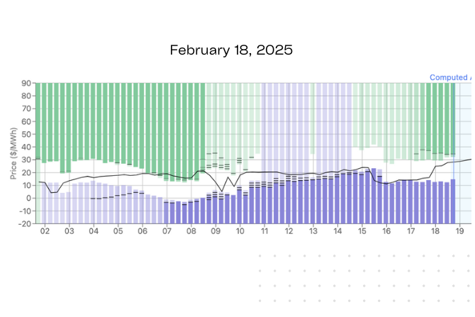
[3] Capitalizing on a seemingly mundane day
Though ERCOT is notorious for its volatility, not every day sees headline-making price spreads. However, there is still revenue that can be made. In the example below, our forecasts predicted a modest peak between 6:45-8:30am. Since the forecasted prices were nothing to write home about, we set opportunistic offers earlier in the morning (see the higher green bars between 4-6am). Why? If we were able to sell into prices higher than those we were forecasting for later in the morning – of course we could want to take advantage of them.
Since those didn’t clear on this day, as we got closer to the forecasted peak, the discharge zone (green bars) dropped into the range that we expected the peak to clear at so we were able to sell into the actual peak.
This way, we net a small profit in the morning, and were in the market in the event prices were unexpectedly high earlier.
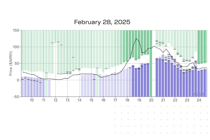
[4] Getting the highest highs / lowest lows
When prices are erratic — rising and falling frequently within a short window, but without any significant spikes or dips – PQ is uniquely able to identify if there will be a price spread large enough to justify cycling the asset. It also helps ensure you charge into the lowest priced intervals, and discharge into the highest.
In this example, prices remained within a ~$50 range throughout the day. With tighter price spreads, the optimizer submitted more bid pairs to maximize the distance between the charge and discharge prices captured. The comparative lows were somewhat random, making them tough to predict. By placing more PQ bid pairs, the asset picked up small amounts of energy when prices were low enough while reserving larger charge volumes for the absolute lowest points – whenever they occurred.
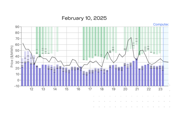
From ~11:30-17:45, prices were generally trending downward. Within this period, the submission of multiple bid pairs enabled the asset to pick up the most charge when prices were at their lowest points – around IE1215 and 1615.
We can see this clearly in the difference between IE12 and 1215. In IE12, prices were ~$40. At this price, we only bid a small amount of capacity (see the price line intersecting with the highest section of the blue bar. By 1215, prices were down around $25, at which price we were charging at full blast (in the bottom most section of the blue bar).
It is also worth zooming in on the period between IE20-2130 as it demonstrates how the PQ structure enables for a more nuanced optimization.
- IE20: We begin discharging a small amount as prices hit our minimum threshold
- IE2015-2045: Discharging increases as prices trend upward of $70
- IE21: Prices suddenly dip and we pick up an opportunistic charge
- IE2115: Prices shoot back up and we are discharging at full blast
Whereas quantity-only bidding would likely have discharged throughout this full period, the agility of the PQ methodology enabled operating optimization.