The exact complexity that makes it challenging to develop and operate high performing energy storage projects is also what makes it difficult to evaluate asset performance. With batteries varying in size, duration, and cycling limits, and nodal price spreads introducing additional variability, determining what “good” looks like isn’t straightforward.
To accurately benchmark performance, we like to look into three categories that compare revenue to peer assets in the market, total revenue opportunity, and simpler operating strategies.
Comparing total revenue to peer assets
Maximizing revenue is a primary objective for many storage operators. To get a high level view of how much revenue individual assets were able to capture across ERCOT – and how your revenue outcomes compare – it can be useful to look at total revenue, by asset.
This data becomes more insightful when we break down the percent of revenue that came from each available product (ex. Real-Time Energy, ECRS, etc.). This way, we can visualize what products were most lucrative and understand if an asset was able to select the best products to sell into at the best times.
To fairly compare performance across different storage assets, we need to normalize for key variables including:
Size and duration:
Look at $/kWh, or hone your sample to only include assets with the same duration (ie. 2-hour) and focused on $/kW.
- An advantage of narrowing in on assets of the same duration is that they will have the same number of shots on goal, so the optimization problem is more analogous.
Cycles:
Looking at $/cycle helps understand cost to value; is incremental revenue from a better strategy, or simply from running the asset more.
Understanding how much of the available revenue opportunity an asset captured
In ERCOT, every node experiences a different amount of volatility. Depending on where an energy storage resource (ESR) is located, it will see different energy prices throughout the day. While a variety of factors contribute to the volatility (or lack thereof), the fact is that certain nodes experience much larger deltas between the highest and lowest prices.
This inherently makes the revenue opportunity across nodes different.
If we take a simple example:
When assessing performance, it is important to normalize for this nodal volatility so you are able to understand if an asset is making the most of the opportunity available. Essentially, we are removing the element of high revenue being misconstrued for optimal performance when it was actually a function of more opportunity.
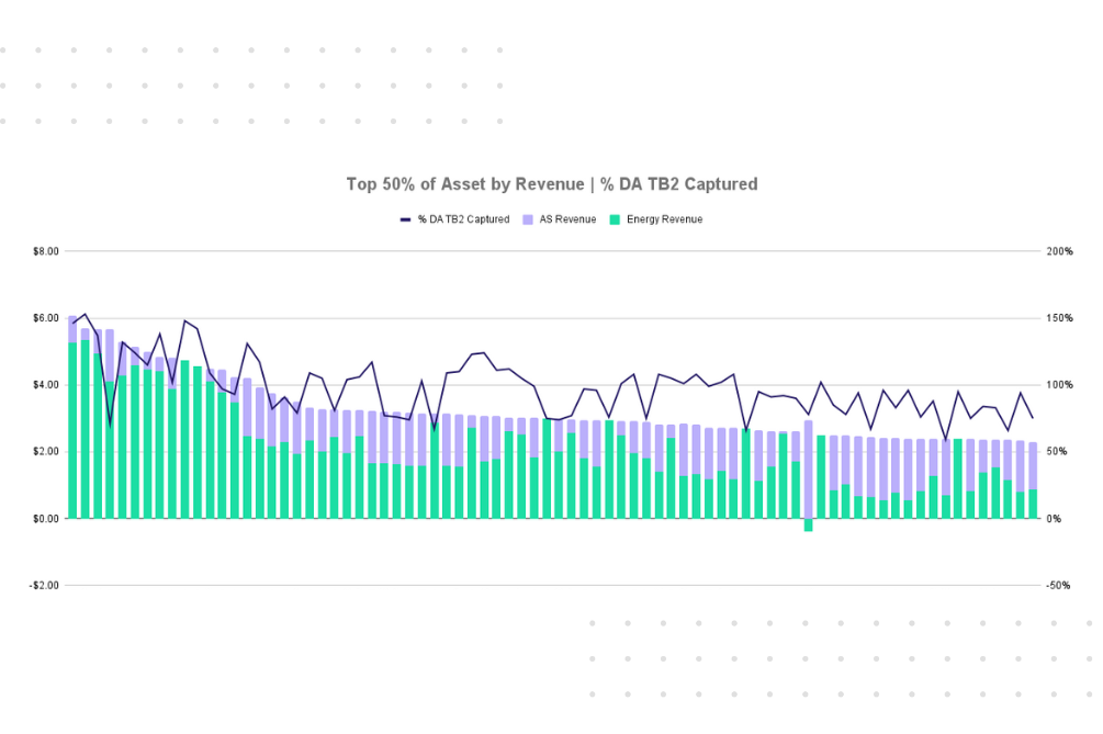
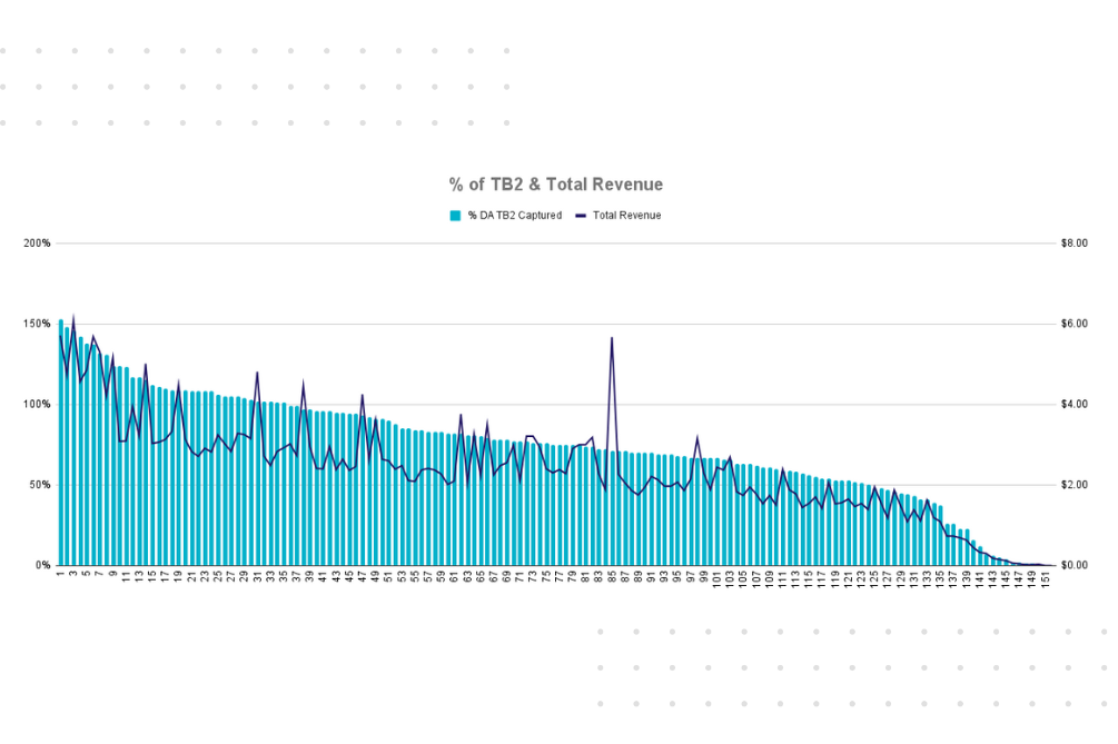
To measure this, we look at the percent of TB2 captured. This metric normalizes for nodal price differences and helps determine whether strong financial performance is due to effective operations or simply a favorable location.
Continuing with the example above, say we are comparing two 100MW storage assets:
While it may have initially appeared as though Asset 1 “performed better,” they actually left a lot of available revenue on the table. In this example, Asset 2 was the better operator as they made more with what they had.
When we add in Ancillary Services (AS), the logic holds.
- AS capacity prices are the same ERCOT wide.
- To simplify, let’s assume AS deployment rates are also the same across ERCOT
- What varies is (1) energy prices and (2) the $/MWh rate at which AS deployment is settled if/when the obligation is called.
- This metric encapsulates the total revenue (across AS and energy) divided by nodal TB2 (revenue opportunity) – so it accurately quantifies how well an asset’s capacity was allocated.
- If an asset allocated more capacity to AS and has a higher percent, we can ascertain that there was less opportunity for energy arbitrage at their node, so they made an optimal tradeoff (ie. the AS capacity payment was more lucrative).
- If an asset allocated more to AS and has a lower %, it missed available arbitrage opportunities.
Ability to maximize the revenue opportunity is most telling of optimal operations.
Comparing revenue outcomes to simple strategies
Finally, we always compare performance to what may have been achievable with less sophisticated, manual operating strategies. If an individual were managing the battery by hand, what could they realistically execute? As a proxy for this, we look at:
-
Energy-only
If you took the DA prices as representative of the highest priced interval and planned to discharge into RT-energy at those times.
-
RRS-only
Assumes clearing 85% of BESS capacity into RRS with no deployment.
These comparisons give us a clear picture of the uplift that more advanced trading strategies unlock. And demonstrates how diversification of revenue streams drives total revenue increases – so long as you are able to optimize efficiently across all products and intervals.
Ultimately, the best operators aren’t just those with the highest total revenue—they’re the ones that consistently maximize the revenue potential of their assets, regardless of location or market conditions.